简介
我们能简单快速的通过scikit-learn获取到鸢尾花数据集(Iris flower dataset)。
因为该数据集比较简单,所以通常会被用在测试或者相关算法的实验。因此我们将在本文中主要使用该数据集。
不过我们只会使用鸢尾花数据集中的两个特征。
数据集拆分及归一化
鸢尾花数据集中包含三种不同鸢尾花的样本,每种花各包含50个样本。同时每个样本包含四个特征,分别是萼片和花瓣的长度和宽度,单位为厘米。
但是,在本文中只使用其中的两种特征
from sklearn import datasets
import numpy as np
iris = datasets.load_iris()
>>> X = iris.data[:,[2,3]]
>>> y = iris.target
为了更好的评判训练后的模型在新数据上的表现,我们会进一步将数据集分成训练数据和测试数据。
>>> from sklearn.cross_validation import train_test_split
>>> X_train, X_test, y_train, y_test = train_test_split(X, y, test_size=0.3, random_state=0)
上面的代码中,我们随机的将 和 分为30%的测试集(45个样本),70%的训练集(105个样本)。
我们同时使用scikit-learn的 Preprocess 模块中 StandardScaler 类来对相关特征做归一化操作,从而优化算法的表现。
>>> from sklearn.preprocessing import StandardScaler
>>> sc = StandardScaler()
>>> sc.fit(X_train)
>>> X_train_std = sc.transform(X_train)
>>> X_test_std = sc.transform(X_test)
从上面的代码中,我们先初始化了 StandardScaler 对象
使用fit 方法,StandardScaler 从训练数据中估计出每个特征的样本均值 , 和样本方差。
然后使用 transform 方法,使用估计得到的 和 来归一化训练样本的特征
同时我们使用相同的参数来归一化测试样本的特征,从而保证训练样本和测试样本的统一。
scikit 感知模型
我们可以使用归一化后的训练集来训练一个感知模型
大多数scikit-learn的算法都支持多分类,通过One-vs-Rest来支持。这样就能让我们将不同类型花的训练数据放入模型中一起训练。
代码如下:
>>> from sklearn.linear_model import Perceptron
>>> ppn = Perceptron(n_iter=40, eta0=0.1, random_state=0)
>>> ppn.fit(X_train_std, y_train)
通过加载linear_model 中的 Perceptron类,我们初始化了一个 Perceptron对象,并通过 fit方法来训练相应的模型。
在这,参数 eta0 就是对应的学习率
其中,如何选择合适的学习率,是需要不断的实验的。
如果学习率过大,算法也许会错过全局最优点。但是如果学习率过小,算法就需要通过更多次的迭代才能达到最终的收敛,这样就导致学习的过程会非常的慢,特别是对于特别大的数据集。
预测
现在我们通过训练得到的模型,使用 predict 方法来对新数据进行预测。
>>> y_pred = ppn.predict(X_test_std)
>>> print('Misclassified samples: %d' % (y_test != y_pred).sum())
Misclassified samples: 18
在这 y_pred 是通过训练模型预测得到的类别标签,y_test 是测试样本对应的真实类别标签。
我们可以看到,感知模型有18个预测错误,那么预测错误率大概是 40% (18/45 ~ 0.4)
同时scikit-learn 还在 metric 模块中提供了多种度量指标。
例如, 我们可以通过下面的方法来计算模型预测的准确率
>>> from sklearn.metrics import accuracy_score
>>> print('Accuracy: %.2f' % accuracy_score(y_test, y_pred))
Accuracy: 0.60
过拟合
我们来了解下机器学习中的一个术语: 过拟合
在统计机器学习中,最普遍的一个任务是通过对训练数据集的拟合出一个模型,然后应用于一些未经训练的数据上。
在过度拟合中,统计模型过度了描述了随机误差和噪声,导致对数据基础关系的描述降低。
过度拟合通常会发生在模型过于复杂,使用过多的变量来描述一个简单的模型。
如果一个模型过度拟合,那么最终的测试表现将会非常的差,主要因为对数据微小的改变,过拟合的模型都会有很大的反应。
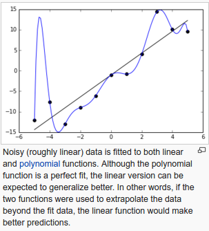
From Overfit wiki
决策区域(decison region)
接下来,我们将根据训练出来的感知模型画出对应的决策区域(decison region),通过可视化的手段来看看模型对不同花的区分效果如何。
from matplotlib.colors import ListedColormap
import matplotlib.pyplot as plt

def plot_decision_regions(X, y, classifier, test_idx=None, resolution=0.02):
   # setup marker generator and color map
   markers = ('s', 'x', 'o', '^', 'v')
   colors = ('red', 'blue', 'lightgreen', 'gray', 'cyan')
   cmap = ListedColormap(colors[:len(np.unique(y))])

   # plot the decision surface
   x1_min, x1_max = X[:, 0].min() - 1, X[:, 0].max() + 1
   x2_min, x2_max = X[:, 1].min() - 1, X[:, 1].max() + 1
   xx1, xx2 = np.meshgrid(np.arange(x1_min, x1_max, resolution),
   np.arange(x2_min, x2_max, resolution))
   Z = classifier.predict(np.array([xx1.ravel(), xx2.ravel()]).T)
   Z = Z.reshape(xx1.shape)
   plt.contourf(xx1, xx2, Z, alpha=0.4, cmap=cmap)
   plt.xlim(xx1.min(), xx1.max())
   plt.ylim(xx2.min(), xx2.max())

   # plot all samples
   X_test, y_test = X[test_idx, :], y[test_idx]
   for idx, cl in enumerate(np.unique(y)):
      plt.scatter(x=X[y == cl, 0], y=X[y == cl, 1],
               alpha=0.8, c=cmap(idx),
               marker=markers[idx], label=cl)
   # highlight test samples
   if test_idx:
      X_test, y_test = X[test_idx, :], y[test_idx]
      plt.scatter(X_test[:, 0], X_test[:, 1], c='',
               alpha=1.0, linewidth=1, marker='o',
               s=55, label='test set')

X_combined_std = np.vstack((X_train_std, X_test_std))
y_combined = np.hstack((y_train, y_test))
plot_decision_regions(X=X_combined_std, y=y_combined,
                      classifier=ppn, test_idx=range(105,150))
plt.xlabel('petal length [standardized]')
plt.ylabel('petal width [standardized]')
plt.legend(loc='upper left')
plt.show()
下面是我们运行后的结果
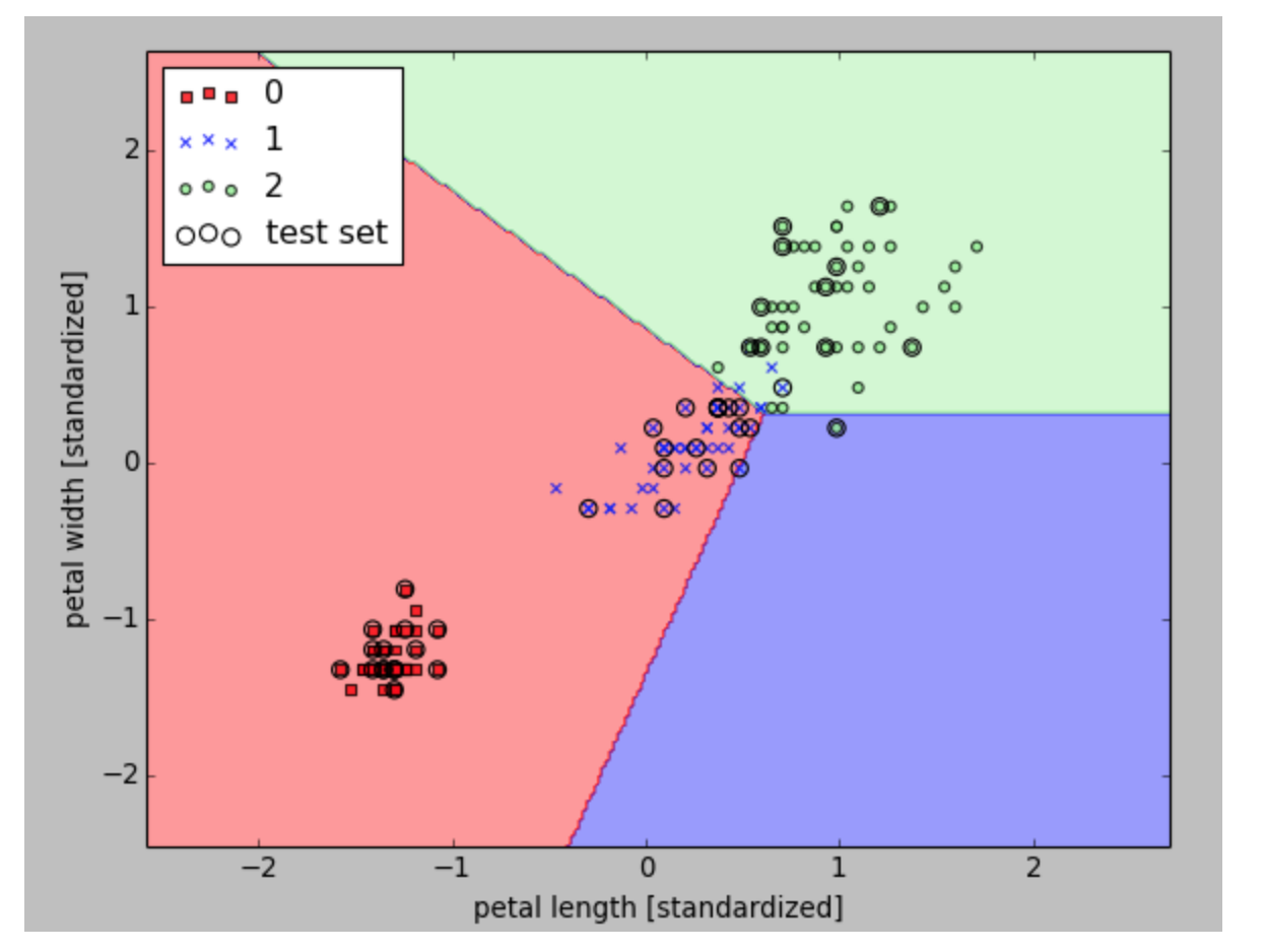
感知算法对于线性不可分的数据收敛的效果非常不好,所以在实践中使用感知算法非常的少。
稍后,我们将会介绍一些更强大的线性分类器。